Reconstructing Computational Paradigms for Pathological Image Analysis
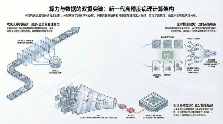 Image credit:
The gigapixel scale of Whole Slide Images (WSI), the chronic absence of clinical multimodal data, and the “compute wall” for fine-tuning large models constitute the “Three Major Hurdles” restricting the development of high-precision pathological AI.
This project reconstructs the computational paradigm of pathological image analysis across three dimensions: low-rank architectural breakthroughs, robust fusion mechanisms for missing modalities, and task-specific efficient fine-tuning.
1. Breaking the “Low-Rank” Bottleneck in Long Sequences (LongMIL)
Original Paper: Rethinking Transformer for Long Contextual Histopathology Whole Slide Image Analysis (NeurIPS 2024) Authors: Honglin Li, Yunlong Zhang, Pingyi Chen, Zhongyi Shui, Chenglu Zhu, Lin Yang
The Scientific Question: The Transformer’s “Achilles’ Heel” in WSI
When processing WSIs containing tens of thousands of patches, traditional Transformers face two critical challenges:
- Explosive Complexity: The $O(N^2)$ complexity of standard Self-Attention makes memory usage unsustainable.
- Low-Rank Bottleneck: We theoretically revealed that when sequence length $N$ far exceeds embedding dimension $D$, the attention matrix exhibits mathematical “low-rank” properties. This means attention maps become homogenized, failing to capture fine-grained local microenvironmental differences.
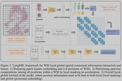
Core Method: Local-Global Hybrid Attention
To break the rank limit and reduce computation, we propose the LongMIL architecture:
- Local Attention Mask: By introducing local window constraints, we force the model to focus on interactions within local neighborhoods. Theory proves this sparsification significantly increases the Rank of the attention matrix.
- Linear Complexity: Utilizing a Chunked Computation strategy reduces complexity from quadratic $O(N^2)$ to linear $O(N \times w)$ (where $w$ is window size).
- Dual-Stream Architecture: A “Local-First, Global-Second” design captures cell community features before aggregating slide-level information.
Results
Table1
Table 2
On BRACS and TCGA-BRCA datasets:
- Performance: F1-score reached 0.657 on BRACS tumor typing, significantly outperforming SOTA methods like TransMIL.
- Extrapolation: In “train small, test large” experiments, LongMIL showed strong robustness (p-value $\approx$ 0.1), proving its adaptability to varying WSI sizes.
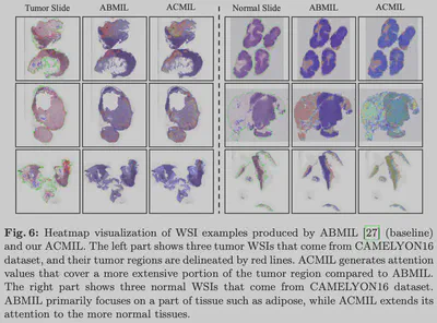
2. Feature Mining under Weak Supervision: Attention-Challenging MIL (ACMIL)
Original Paper: Attention-Challenging Multiple Instance Learning for Whole Slide Image Classification (ECCV 2024) Authors: Yunlong Zhang, Honglin Li, Yunxuan Sun, Sunyi Zheng, Chenglu Zhu, Lin Yang
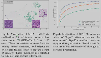
The Scientific Question: Attention “Laziness”
In Weakly Supervised Multiple Instance Learning (MIL), models tend to focus only on the most obvious discriminative regions (e.g., tumor cores), ignoring edges or atypical key features. This “Attention Laziness” leads to poor generalization on heterogeneous tumors.
Core Method: Adversarial Attention Enhancement
We propose the ACMIL framework to “manufacture difficulty” for the model:
- Multi-Branch Attention (MBA): Parallel attention branches capture distinct clustering patterns in the feature space (verified via UMAP), covering more diverse pathological features.
- Stochastic Top-K Instance Masking (STKIM): During training, we randomly “mask” the Top-K instances with the highest attention scores.
Results
- Camelyon16: Achieved an AUC of 0.954, outperforming methods like DTFD-MIL.
- TCGA-LBC: AUC increased to 0.901 on liquid-based cytology data, proving effectiveness in sparse feature mining.
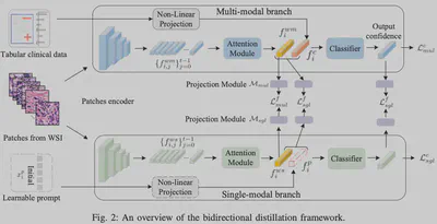
3. Addressing Missing Clinical Data: Bidirectional Distillation
Original Paper: Multi-modal Learning with Missing Modality in Predicting Axillary Lymph Node Metastasis (BIBM 2023) Authors: Shichuan Zhang, Sunyi Zheng, Zhongyi Shui, Honglin Li, Lin Yang
The Scientific Question: The Multimodal “Bucket Effect”
In clinical practice, WSI and tabular data (genomics, clinical markers) are often asynchronous. Existing multimodal models often suffer a severe performance drop—sometimes below single-modal baselines—when clinical data is missing.
Core Method: Bidirectional Distillation & Learnable Prompts
We propose a Bidirectional Distillation (BD) framework to teach the model how to handle missingness:
- Decoupling: Parallel “Single-Modal Branch” (WSI only) and “Multi-Modal Branch” (WSI + Clinical).
- Learnable Prompt: A learnable vector acts as a placeholder for missing modalities in the single-modal branch.
- Bidirectional Distillation: We distill fused knowledge from Multi $\to$ Single ($\mathcal{M} \to \mathcal{S}$) and distill pure image features back from Single $\to$ Multi ($\mathcal{S} \to \mathcal{M}$) to prevent noise interference.
Results
In BCNB Breast Cancer Lymph Node Metastasis prediction:
- Resilience: With 80%-100% clinical data missing, BD maintained an F1-score of ~74.9%, while direct filling methods crashed to below 68%.
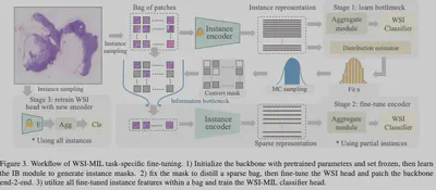
4. Low-Cost WSI Adaptation: Variational Information Bottleneck Fine-tuning
Original Paper: Task-specific Fine-tuning via Variational Information Bottleneck for Weakly-supervised Pathology Whole Slide Image Classification (CVPR 2023) Authors: Honglin Li, Chenglu Zhu, Yunlong Zhang, Yuxuan Sun, Zhongyi Shui, Wenwei Kuang, Sunyi Zheng, Lin Yang
The Scientific Question: The WSI “Compute Wall”
Pathology models typically use ImageNet pre-trained backbones, which suffer from a domain gap. However, end-to-end full fine-tuning on WSIs (thousands of patches) requires VRAM far beyond standard GPU capabilities.
Core Method: Sparse Critical Instance Selection
Based on Variational Information Bottleneck (VIB) theory, we screen for the “minimal sufficient statistics”:
- IB Module Screening: A lightweight module selects the Top-K diagnostic instances (usually <1000) based on mutual information maximization.
- Sparse Backpropagation: Gradients are back-propagated only through selected instances during fine-tuning, reducing computational overhead by >10x.
Results
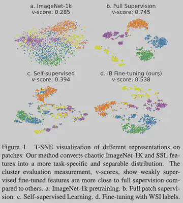
- Performance Leap: On Camelyon16, a VIB fine-tuned ResNet-50 with simple Max-pooling achieved an AUC of 0.969, a 14.5% jump over the ImageNet baseline (0.824).
- Feature Space: t-SNE visualization confirms significantly improved inter-class separation.
Summary
This research directly targets the “compute” and “data” bottlenecks in pathological AI deployment.
- LongMIL & ACMIL reconstruct WSI attention mechanisms.
- BD Framework solves the pain point of missing clinical data.
- VIB Fine-tuning breaks the compute barrier for large-scale model optimization.
Together, these provide the core algorithmic support for building high-precision, low-cost, and robust pathological AI systems.